# =============================================================================
# Separate PLS Models Per Target
# =============================================================================
#
# Training one PLS model per target allows:
# - Better interpretability: each target has its own loadings showing which
# spectral regions are important for that specific compound
# - Independent optimization: each target can have its own optimal number of
# components
# - Potentially better performance: models can focus on the specific spectral
# regions relevant to each compound
target_names = ["glucose", "Na_acetate", "Mg_SO4"]
target_models = {}
target_optimal_components = {}
target_metrics_separate = {}
target_predictions_separate = {}
# Store single model metrics for comparison (from cell 11)
target_metrics_single = {}
for i, target_name in enumerate(target_names):
Y_target = Y[:, i]
y_pred_target = y_pred_final[:, i]
r2_target = r2_score(Y_target, y_pred_target)
rmse_target = root_mean_squared_error(Y_target, y_pred_target)
target_metrics_single[target_name] = (r2_target, rmse_target)
# Train separate PLS model for each target
for target_idx, target_name in enumerate(target_names):
print(f"\n{'='*60}")
print(f"Training PLS model for {target_name}")
print(f"{'='*60}")
# Extract single target
Y_target = Y[:, target_idx].reshape(-1, 1) # Reshape to (n_samples, 1)
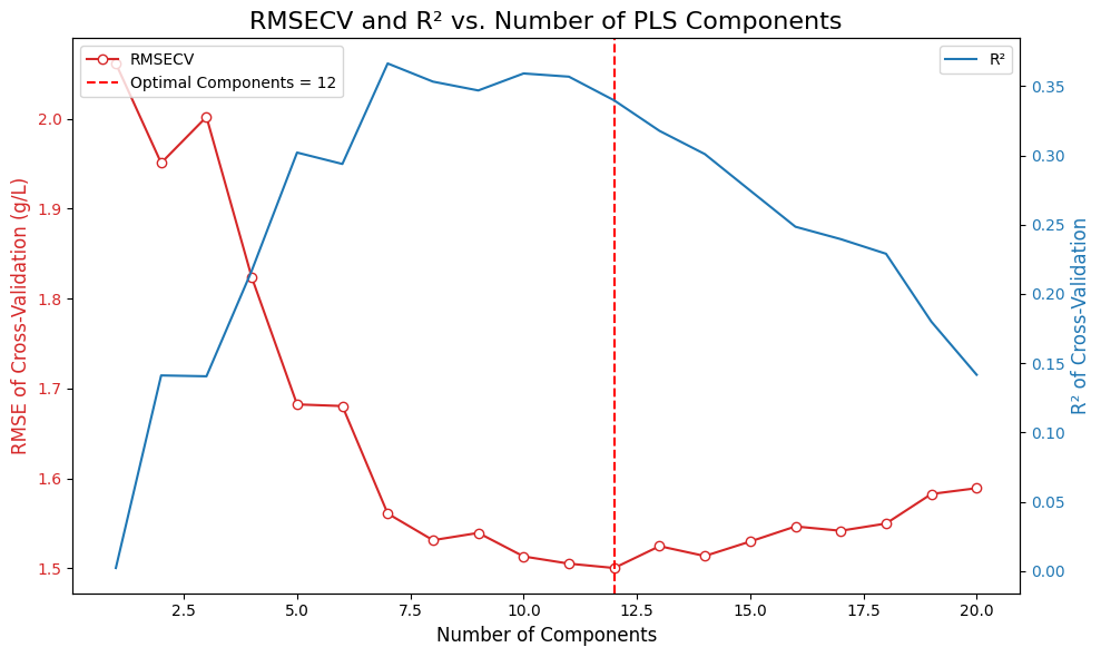
# Find optimal number of components for this target
n_components_range = np.arange(1, 21)
rmsecv_scores = []
r2cv_scores = []
for n_comp in n_components_range:
pls = PLSRegression(n_components=n_comp)
y_pred_cv = cross_val_predict(pls, X_processed, Y_target, cv=cv_splitter, groups=groups)
rmsecv = root_mean_squared_error(Y_target, y_pred_cv)
r2cv = r2_score(Y_target, y_pred_cv)
rmsecv_scores.append(rmsecv)
r2cv_scores.append(r2cv)
print(f" {n_comp:2d} components: RMSECV={rmsecv:.4f}, R²CV={r2cv:.4f}")
# Find optimal number of components
optimal_n_components = n_components_range[np.argmin(rmsecv_scores)]
target_optimal_components[target_name] = optimal_n_components
print(f"\n Optimal components for {target_name}: {optimal_n_components}")
# Train final model and get cross-validated predictions
final_pls = PLSRegression(n_components=optimal_n_components)
y_pred_final_separate = cross_val_predict(final_pls, X_processed, Y_target, cv=cv_splitter, groups=groups)
# Calculate metrics
r2_final = r2_score(Y_target, y_pred_final_separate)
rmse_final = root_mean_squared_error(Y_target, y_pred_final_separate)
target_metrics_separate[target_name] = (r2_final, rmse_final)
target_models[target_name] = final_pls
target_predictions_separate[target_name] = y_pred_final_separate
print(f" Final R²: {r2_final:.4f}, RMSE: {rmse_final:.4f} g/L")
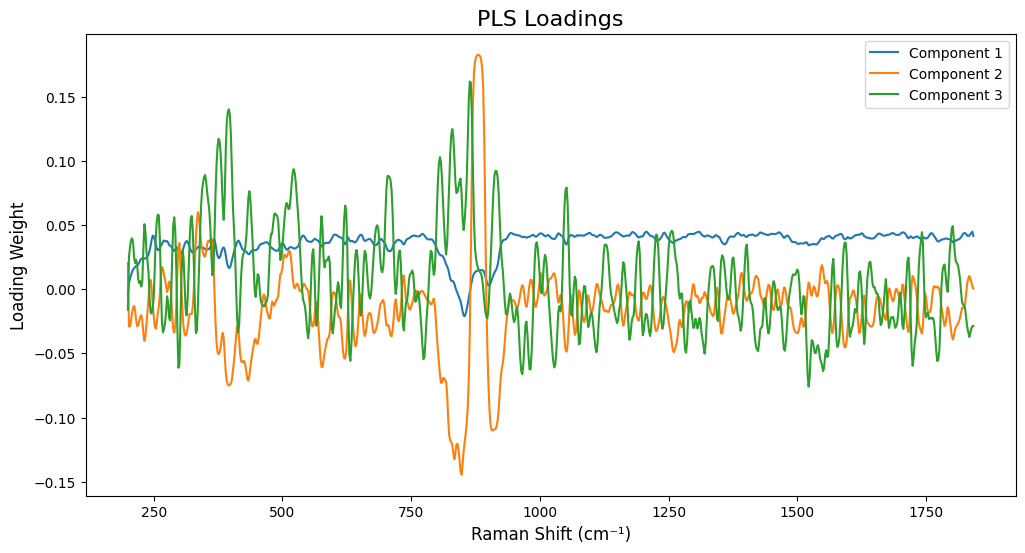
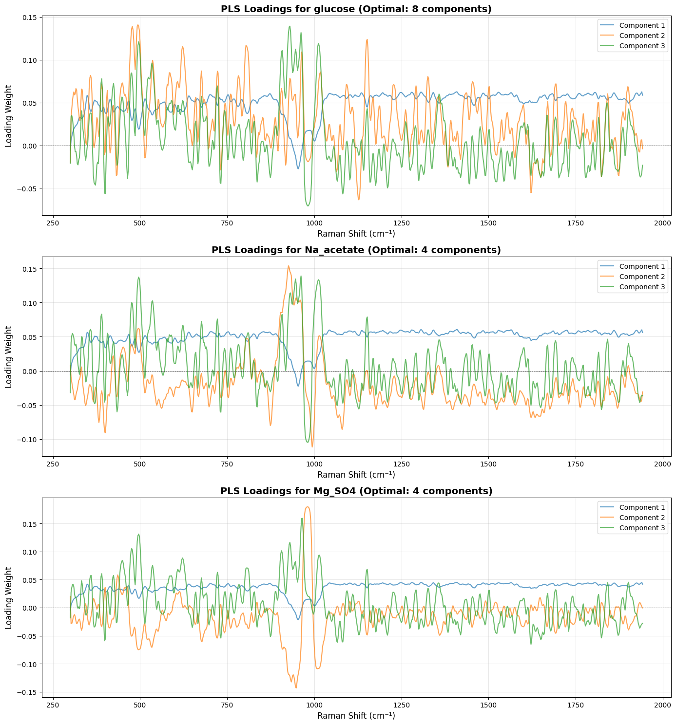
# =============================================================================
# Plot Loadings for Each Target (Much More Interpretable!)
# =============================================================================
fig, axes = plt.subplots(len(target_names), 1, figsize=(14, 5*len(target_names)))
# Handle case where we have only one target (axes would be 1D, not 2D)
if len(target_names) == 1:
axes = [axes]
for idx, target_name in enumerate(target_names):
model = target_models[target_name]
# Fit the model on all data to get loadings
model.fit(X_processed, Y[:, idx].reshape(-1, 1))
loadings = model.x_loadings_
# Use wavenumbers from processed spectra to match loadings dimensions
wavenumbers_processed = processed_spectra.spectral_axis
if hasattr(wavenumbers_processed, 'values'):
wavenumbers_processed = wavenumbers_processed.values
ax = axes[idx]
n_comp_to_plot = min(3, target_optimal_components[target_name])
for comp_idx in range(n_comp_to_plot):
ax.plot(wavenumbers_processed, loadings[:, comp_idx],
label=f'Component {comp_idx+1}', alpha=0.7, linewidth=1.5)
ax.set_title(f'PLS Loadings for {target_name} (Optimal: {target_optimal_components[target_name]} components)',
fontsize=14, fontweight='bold')
ax.set_xlabel('Raman Shift (cm⁻¹)', fontsize=12)
ax.set_ylabel('Loading Weight', fontsize=12)
ax.legend(loc='best')
ax.grid(True, alpha=0.3)
ax.axhline(y=0, color='k', linestyle='--', linewidth=0.5)
plt.tight_layout()
plt.show()
# =============================================================================
# Performance Comparison: Single vs. Separate Models
# =============================================================================
print("\n" + "="*80)
print("Performance Comparison: Single Multi-Output Model vs. Separate Models")
print("="*80)
print(f"{'Target':<15} {'Single Model R²':<18} {'Separate Model R²':<18} {'R² Improvement':<15} {'Single RMSE':<15} {'Separate RMSE':<15} {'RMSE Improvement':<15}")
print("-"*80)
for target_name in target_names:
single_r2, single_rmse = target_metrics_single[target_name]
separate_r2, separate_rmse = target_metrics_separate[target_name]
r2_improvement = separate_r2 - single_r2
rmse_improvement = single_rmse - separate_rmse # Positive = better (lower RMSE)
print(f"{target_name:<15} {single_r2:>17.4f} {separate_r2:>17.4f} {r2_improvement:>+14.4f} {single_rmse:>14.4f} g/L {separate_rmse:>14.4f} g/L {rmse_improvement:>+14.4f} g/L")
print("="*80)
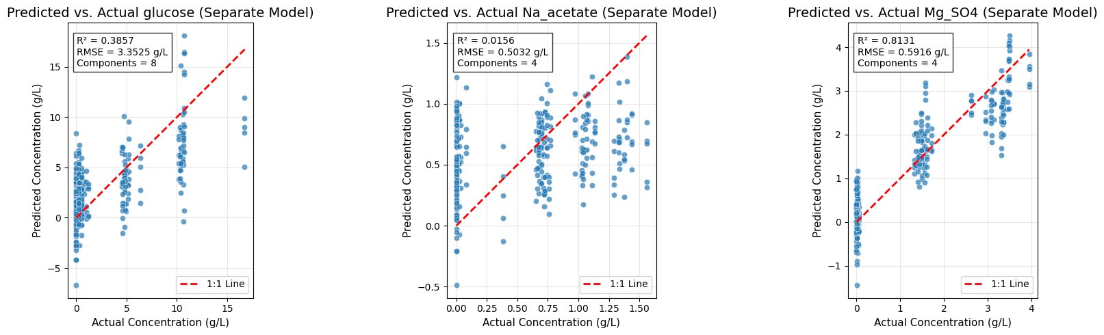
# =============================================================================
# Predicted vs. Actual Plots for Separate Models
# =============================================================================
fig, axes = plt.subplots(1, 3, figsize=(18, 5))
for idx, (target_name, ax) in enumerate(zip(target_names, axes)):
Y_target = Y[:, idx]
y_pred_target = target_predictions_separate[target_name].flatten()
r2_target, rmse_target = target_metrics_separate[target_name]
sns.scatterplot(x=Y_target, y=y_pred_target, alpha=0.7, ax=ax)
ax.plot([Y_target.min(), Y_target.max()], [Y_target.min(), Y_target.max()],
'r--', lw=2, label='1:1 Line')
ax.set_title(f'Predicted vs. Actual {target_name} (Separate Model)', fontsize=14)
ax.set_xlabel('Actual Concentration (g/L)', fontsize=11)
ax.set_ylabel('Predicted Concentration (g/L)', fontsize=11)
ax.text(0.05, 0.95, f'R² = {r2_target:.4f}\nRMSE = {rmse_target:.4f} g/L\nComponents = {target_optimal_components[target_name]}',
transform=ax.transAxes, fontsize=10,
bbox=dict(facecolor='white', alpha=0.8), verticalalignment='top')
ax.legend()
ax.grid(True, alpha=0.3)
ax.set_aspect('equal', adjustable='box')
plt.tight_layout()
plt.show()