This blog post compares two different methods for encoding distances in 3D molecules and protein pockets: Gaussian kernel with pair type (GBFPT) and Discretization categorical embedding with Pair Type (DCEPT). We analyze their performance within the Uni-Mol framework, a universal 3D molecular representation learning model. We observed unstable gradients with GBFPT and hypothesized that DCEPT, inspired by AlphaFold’s distance representation, might offer a more stable alternative. We found that while DCEPT exhibits more stable training behavior, GBFPT ultimately yields superior pocket embeddings for retrieval tasks.
Before diving into the details, let’s define the acronyms used in this article:
- GBFPT: Gaussian Basis Function with Pair Type
- DCEPT: Discretization Categorical Embedding with Pair Type
Introduction to Uni-Mol and Distance Encoding
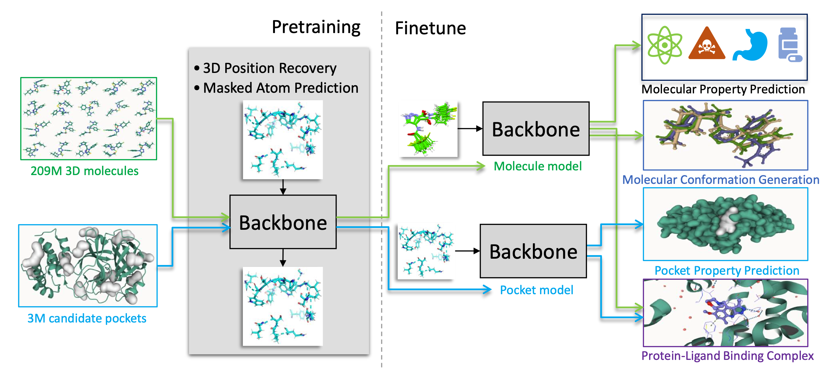
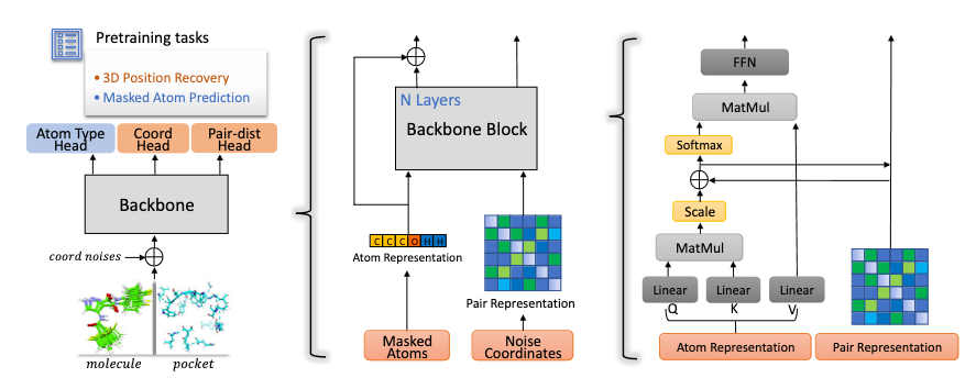
Code for Uni-Mol is available at https://github.com/dptech-corp/Uni-Mol, and the related article is (Zhou et al. 2023). In brief, Uni-Mol is a 3D foundation model for molecules and pockets based on a SE(3) Transformer architecture. It comprises two pretrained models: one for molecular conformations and another for protein pocket data. Uni-Mol is pretrained on large-scale unlabeled data and is able to directly take 3D positions as both inputs and outputs. Uni-Mol backbone is a Transformer based model that can capture the input 3D information and predict 3D positions directly. Uni-Mol pretraining is done on two large-scale datasets: a 209M molecular conformation dataset and a 3M candidate protein pocket dataset, for pretraining 2 models on molecules and protein pockets, respectively. In the pretraining phase, Uni-Mol has to predict masked atoms, as well as masked noisy atoms coordinates and distances for effectively learning 3D spatial representation. The overall pretraining architecture is illustrated in Figure 2 and the framework is given in Figure 1 (taken from (Zhou et al. 2023)).
Background: 3D Spatial Encoding in Uni-Mol
We focus here on the encoding of the coordinates in distances (pair representation in Figure 2 middle part) and the decoding part, prediction of distances (pair-dist head in Figure 2 left part). In (Zhou et al. 2023) Section D.1, 3D spatial positional encodings benchmark, they investigate the performance of different 3D spatial positional encoding on the 3D molecular pretraining. In particular, they benchmarked:
Gaussian kernel (GK), a simply Gaussian density function.
Gaussian kernel with pair type (GKPT) (Shuaibi et al. 2021). Based on GK, an affine transformation according to the pair type is applied on pair distances, before applying the Gaussian kernel.
Radial Bessel basis (RBB) (Gasteiger, Yeshwanth, and Günnemann 2021). A Bessel based radial function.
Discretization categorical embedding (DCE). They convert the continued distances to the discrete bins, by Discretization. With binned distances, embedding-based positional encoding is directly used.
Delta coordinate (DC) (Zhao et al. 2021). Following Point Transformer, the deltas of coordinates are directly used as pair-wise spatial relative positional encoding.
Gaussian kernel with pair type and local graph (GKPTLG). Based on GKPT, they set up a model with locally connected graphs. In particular, the cutoff radius is set to 6 Å.
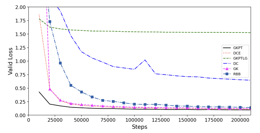
The validation loss during pretraining for each encoding is summarized in Figure 3 (taken from (Zhou et al. 2023)). From the results, they drew the following conclusions:
The performance of DCE and GK are almost the same, and outperform RBB and DC. And they choose GK as the basic encoding.
Compared with GK, GKPT converges faster. This indicates the pair type is critical in the 3D spatial positional encoding.
Compared with GKPT, GKPTLG converges slower. This indicates the locally cutoff graph is not effective for self-supervised learning, and the default fully connected graph structure inherent in the Transformer architecture is more effective.
As GKPT outperforms all other encoding, they use it in the backbone model of Uni-Mol.
The code for the GKPT encoding is given by:
import torch
import torch.nn as nn

@torch.jit.script
def gaussian(x, mean, std):
    pi = 3.14159
    a = (2 * pi) ** 0.5
    return torch.exp(-0.5 * (((x - mean) / std) ** 2)) / (a * std)


class GaussianLayer(nn.Module):
    def __init__(self, K=128, edge_types=1024):
        super().__init__()
        self.K = K
        self.means = nn.Embedding(1, K)
        self.stds = nn.Embedding(1, K)
        self.mul = nn.Embedding(edge_types, 1)
        self.bias = nn.Embedding(edge_types, 1)
        nn.init.uniform_(self.means.weight, 0, 3)
        nn.init.uniform_(self.stds.weight, 0, 3)
        nn.init.constant_(self.bias.weight, 0)
        nn.init.constant_(self.mul.weight, 1)

    def forward(self, x, edge_type):
        mul = self.mul(edge_type).type_as(x)
        bias = self.bias(edge_type).type_as(x)
        x = mul * x.unsqueeze(-1) + bias
        x = x.expand(-1, -1, -1, self.K)
        mean = self.means.weight.float().view(-1)
        std = self.stds.weight.float().view(-1).abs() + 1e-5
        return gaussian(x.float(), mean, std).type_as(self.means.weight)
K represents the number of Gaussian basis functions, edge_types the number of possible edge types, x the distance matrix (for an initial 3D molecule or pocket) and edge_type the corresponding edge type matrix. Edge types represent the different types of atom pairs (e.g., C-C, C-O, C-N, etc.)
Experimental Setup
All the Uni-Mol experiments run for this article are based on a small pockets dataset inspired from the PDBbind database (http://www.pdbbind.org.cn/), a collection of protein-ligand complexes and their binding affinities. The dataset was split into training and validation sets based on pocket similarity. The wandb project is available https://wandb.ai/nicolasb/unimol_analysis/ as well as a summary report https://api.wandb.ai/links/nicolasb/kdz59bry.
Motivation for DCEPT and Implementation
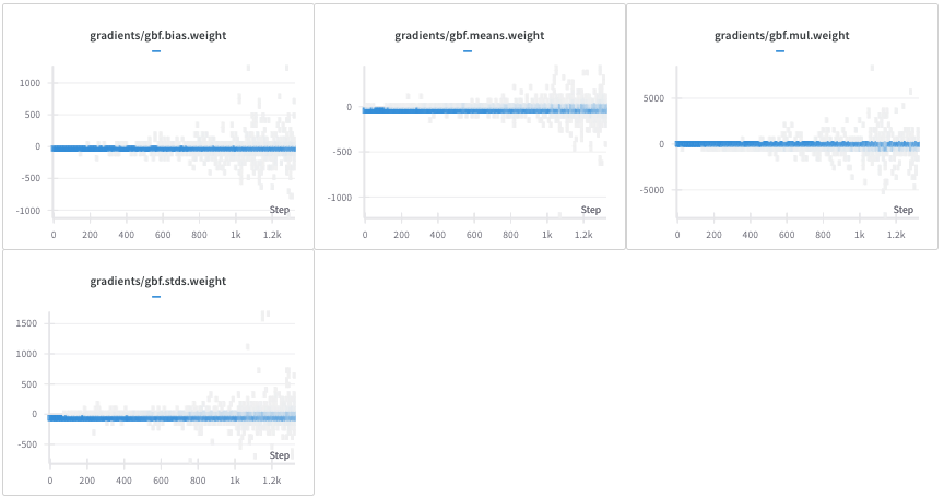
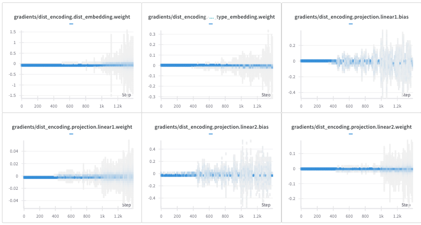
When we train Uni-Mol on a small dataset of pockets inspired from the PDBbind database, we remark that the gradients related to GaussianLayer parameters are not stable and can take very large values. To address the gradient instability observed with GBFPT, and drawing inspiration from AlphaFold’s use of discretization, we explored using a Discretization Categorical Embedding with Pair Type (DCEPT) as an alternative. In Figure 4, some gradients are of the order of one thousand. Uni-Mol relies on Uni-Core which implements gradient clipping and these high values do not affect the stability of the training.
Nevertheless, we wanted to try another encoding that would be naturally stable without exploding gradients. Furthermore, DCE is the encoding used in AlphaFold (Jumper et al. 2021). We implemented Discretization categorical embedding with Pair Type encoding (DCEPT) that takes into account the edge type. A distogram is a discrete representation of the distance matrix, where distances are binned into predefined intervals. The binning process transforms continuous distances into discrete categories.
import torch
import torch.nn as nn

# Constants
PAD_DIST = 0

class NonLinearModule(nn.Module):
    def __init__(self, input_dim, out_dim, activation_fn):
        super().__init__()
        self.linear = nn.Linear(input_dim, out_dim)
        self.activation = getattr(nn, activation_fn)()

    def forward(self, x):
        return self.activation(self.linear(x))

class DistEncoding(nn.Module):
    def __init__(
        self,
        distogram_nb_bins: int,
        nb_edge_types: int,
        embedding_dim: int,
        edge_type_padding_idx: int,
        encoder_attention_heads: int,
        activation_fn: str,
    ):
        """
        Initializes the DistEncoding module for encoding distances and edge types.

        Args:
            distogram_nb_bins: Number of bins for the distogram (distance discretization).
            nb_edge_types: Number of possible edge types (e.g., different bond types).
            embedding_dim: Dimension of the embeddings for distances and edge types.
            edge_type_padding_idx: Padding index for edge type embeddings.
            encoder_attention_heads: Number of attention heads in the Transformer encoder.
            activation_fn: Activation function to use in the projection layer.
        """
        super(DistEncoding, self).__init__()

        # Embedding layer for the distogram (discretized distances)
        self.dist_embedding = nn.Embedding(
            num_embeddings=distogram_nb_bins,
            embedding_dim=embedding_dim,
            padding_idx=PAD_DIST,  # Use PAD_DIST for padding
        )

        # Embedding layer for edge types
        self.edge_type_embedding = nn.Embedding(
            num_embeddings=nb_edge_types,
            embedding_dim=embedding_dim,
            padding_idx=edge_type_padding_idx,
        )

        # Projection layer to combine distance and edge type embeddings and project
        # to the correct dimension for attention bias.
        self.projection = NonLinearModule(
            input_dim=2 * embedding_dim,  # Concatenate dist and edge embeddings
            out_dim=encoder_attention_heads,  # Output dimension matches attention heads
            activation_fn=activation_fn,
        )

    def forward(
        self, distogram: torch.Tensor, edge_types: torch.Tensor
    ) -> torch.Tensor:
        """
        Forward pass of the DistEncoding module.

        Args:
            distogram: Tensor of discretized distances (batch_size, seq_len, seq_len).
            edge_types: Tensor of edge types (batch_size, seq_len, seq_len).

        Returns:
            attn_bias: Tensor of attention biases (batch_size, num_heads, seq_len, seq_len).
        """
        n_node = distogram.size(-1)  # Sequence length (number of nodes/atoms)

        # Embed the discretized distances
        dist_embeddings = self.dist_embedding(distogram)  # (B, L, L, D)

        # Embed the edge types
        edge_types_embeddings = self.edge_type_embedding(edge_types)  # (B, L, L, D)

        # Concatenate distance and edge type embeddings
        embeddings = torch.cat((dist_embeddings, edge_types_embeddings), dim=-1)  # (B, L, L, 2D)

        # Project the combined embeddings to generate attention bias
        attn_bias = self.projection(embeddings)  # (B, L, L, H) where H = num_heads

        # Reshape the attention bias to the correct format for the Transformer
        attn_bias = attn_bias.permute(0, 3, 1, 2).contiguous()  # (B, H, L, L)
        attn_bias = attn_bias.view(-1, n_node, n_node) # (B*H, L, L) - Correct if attention is applied per head.
        return attn_bias
distogram_nb_bins is the number of bins (128 by default), nb_edge_types the number of edge types, embedding_dim the dimension of the embedding (128 by default), encoder_attention_heads the number of attention heads in the transformer because the distance encoding is directly injected in the attention matrix. distogram is the distogram (discretization of the distance matrix) and edge_types the edge types. We concatenate the two embeddings creating de facto the DCEPT and then project to feed into the attention matrix.
Training Dynamics
During the training, the gradients related to DistEncoding parameters do not take large values and are naturally stable without clipping gradients. This is illustrated in Figure 5.
Following (Jumper et al. 2021) distogram prediction task, we also replace the distance prediction task (mean squared error loss) implemented in Uni-Mol by a distogram prediction task (cross entropy loss). We remark that this loss replacement does not change the characteristics of Uni-Mol.
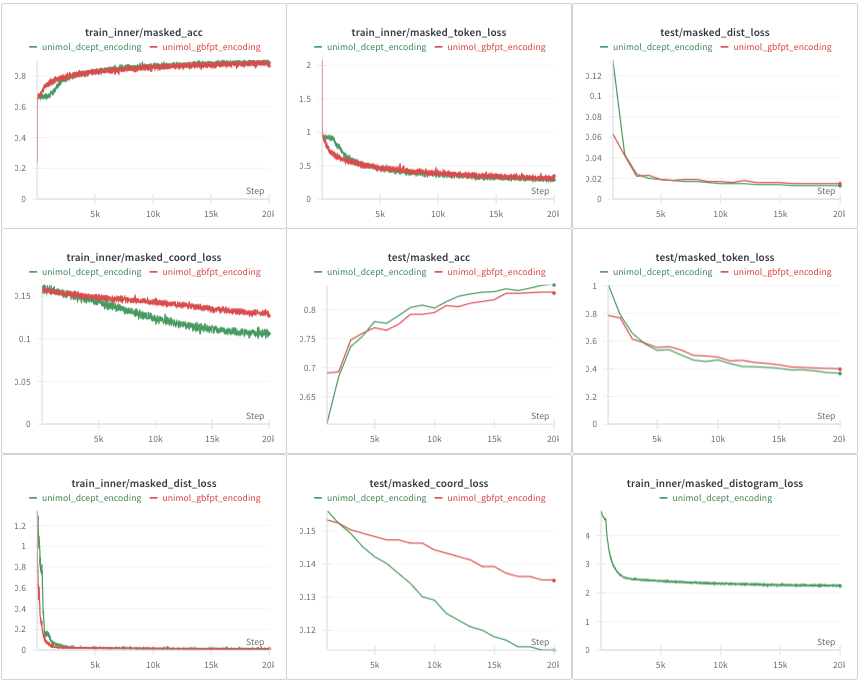
On the small pockets inspired from the PDBbind database, we notice that the training and validation loss curves are better with DCEPT encoding compared to GBFPT encoding (on average), see Figure 6. More precisely, the masked_token_loss and the masked_acc metrics related to the recovery of masked atoms seem to stagnate a little at first with DCEPT encoding compared to GBFPT encoding. It may be due to the fact that DCEPT are at first completely random embeddings and less intuitive for the neural network. However, the masked_coord_loss is better with DCEPT encoding both in the training and validation sets. Note that the masked_distogram_loss corresponds to the distogram loss (cross entropy loss) used in AlphaFold (Jumper et al. 2021) and is implemented only for DCEPT encoding. For DCEPT encoding, we also add a distance prediction head with the corresponding MSE loss taken from Uni-Mol and a small multiplication factor (0.01). The rationale for including this head was to maintain some of the original Uni-Mol distance prediction capabilities alongside the distogram prediction. That explains why the DCEPT masked_dist_loss decreases slightly slower than GBFPT. Several additional experiments (not shown here) demonstrate that using a distogram or distance loss does not change the behavior of Uni-Mol.
In conclusion, according to the loss curves and the stability of the gradients, DCEPT seems to be a better encoding than GBFPT (or at least as good as) during pre-training.
Downstream Performance: Pocket Retrieval
However, Uni-Mol stands as a foundational model pre-trained through unsupervised methods. The pre-training metrics do not reflect the expected capabilities of the model. Notably, we expect that the pockets embeddings obtained with Uni-Mol should be good proxies of the pockets themselves: if two pockets are close to each other, their embeddings should be close in cos similarity or euclidean distance.
We have collected a dataset of 5 pockets (taken from 2oax, 3oxc, 5kxi, 5zk3 and 6v7a proteins) and for each pocket, a group of similar and dissimilar pockets. We compute the cos similarities between each reference pocket and the similar/dissimilar pockets and we sort the pockets by their cos similarity. Better embeddings translate into more similar pockets in the top retrieved pockets. More precisely, we sort the pockets by their cos similarities, we select the top 100 pockets, we count the number of similar pockets in the top 100 and we get a number between 0 and 1, the higher the better. We test two different embeddings: either, the vector corresponding to the [CLS] token (see (Zhou et al. 2023) Section 2.2) (indicated by _cls) or the mean of the pocket atoms vectors (indicated by _mean). Table 1 summarizes the results for each encoding, embedding and reference pocket and we remark that
GBFPT is superior to DCEPT for pockets retrieval,
The mean of the pocket atoms vectors is better or near as good as the
[CLS]embedding.
| 6v7a | 2oax | 5kxi | 5zk3 | 3oxc | |
|---|---|---|---|---|---|
| unimol_gbfpt_cls | 0.46 | 1.0 | 0.32 | 0.3 | 1.0 |
| unimol_gbfpt_mean | 0.79 | 1.0 | 0.38 | 0.29 | 1.0 |
| unimol_dcept_cls | 0.3 | 1.0 | 0.26 | 0.29 | 1.0 |
| unimol_dcept_mean | 0.51 | 1.0 | 0.27 | 0.28 | 1.0 |
Investigating Noise Sensitivity
In conclusion, despite better pre-training behavior and metrics, DCEPT encoding is disappointing when it comes to embeddings comparison. We suppose that this defect comes from a higher sensitivity of the discretization procedure. Two distance matrices from two close pockets may be more distinctly differentiated with DCEPT encoding compared to GBFPT encoding. This could be due to the information loss inherent in discretizing continuous distances. GBFPT might be capturing subtle long-range interactions that DCEPT, with its discrete representation, misses. To test this hypothesis, we take the 6v7a pocket and we noise its coordinates with a uniform noise between 0 and 1A. Since we have a batch size of 16, we fill up a batch with the reference pocket 6v7a and 15 noisy pockets. For each pocket, the distance matrix is encoded by GBFPT or DCEPT and we get an encoding of size 128 for each distance in the distance matrix. We compute the cos similarities between each encoding and the reference encoding in the reference matrix distance of 6v7a and we obtain the overall statistics of these cos similarities for GBFPT and DCEPT. In Table 2, we have the absolute errors statistics between 1 and the cos similarities of the noisy pockets from 6v7a, the lower the better because the vectors are similar. We remark that as presumed DCEPT encoding is less robust to noise compared to GBFPT encoding.
| Absolute errors cos similarities GBFPT encoding (1 - cos similarities) | Absolute errors cos similarities DCEPT encoding (1 - cos similarities) | |
|---|---|---|
| mean | 0.002 | 0.020 |
| median | 0.000 | 0.007 |
Conclusion
These results suggest that while DCEPT offers advantages during pre-training in terms of gradient stability, the discretization process might lead to a loss of information and reduced robustness, ultimately hindering the quality of the generated pocket embeddings for downstream tasks like pocket retrieval. Further research is needed to investigate the optimal bin size for distograms and to explore alternative distance encoding techniques that balance stability and information retention. This analysis was conducted on a small, custom-built pocket dataset, and future work should evaluate these encoding methods on larger, more diverse datasets to ensure the generalizability of our findings.
References
Citation
@online{brosse2024,
  author = {Brosse, Nicolas},
  title = {Encoding {Distances} in {Molecules} and {Pockets:} {A}
    {Comparison} of {GBFPT} and {DCEPT}},
  date = {2024-04-24},
  url = {https://nbrosse.github.io/posts/encoding-distances/unimol-gbf.html},
  langid = {en}
}