This note follows and extends the perspective of (Holderrieth and Erives 2025; Lipman et al. 2024). It also builds on the code and analysis of (Holderrieth and Erives 2026), using their flow-matching setup as a starting point.
The central object in flow matching is the marginal velocity field. Conditional flow matching gives us a convenient training target, but the vector field that the model should learn is not the conditional target itself. It is a posterior average of conditional targets.
The goal of this note is to make that statement concrete in a simple example. The example is intentionally low-dimensional: the data distribution is a symmetric five-component Gaussian mixture in dimension two, the reference distribution is standard Gaussian, and the conditional probability path is Gaussian, \[ X_t = \alpha_t Z + \beta_t \varepsilon, \qquad Z \sim p_{\mathrm{data}}, \qquad \varepsilon \sim \mathcal{N}(0,I_d). \] This setting is simple enough to visualize, but still rich enough to show the main difficulty: at intermediate times, the posterior distribution of the endpoint \(Z\) given the current state \(X_t=x\) can be multimodal.
The accompanying code is available on GitHub. The main experiment is implemented in the notebook.
The note has three aims:
- Derive the marginal velocity field for Gaussian probability paths.
- Show that, for a Gaussian-mixture data distribution, the posterior \(p_t(z\mid x)\) and the marginal velocity are available in closed form.
- Explain the difference between the FM and CFM losses as an irreducible posterior-variance term due to posterior uncertainty about the endpoint \(Z\).
Introduction and notation
We work in \(\mathbb{R}^d\). In the numerical experiment later on, \(d=2\). Let \(Z\sim p_{\mathrm{data}}\) denote a data point. In the running experiment, \(p_{\mathrm{data}}\) is a two-dimensional five-component Gaussian mixture. The reference distribution is \[ p_{\mathrm{simple}} = \mathcal{N}(0,I_d). \]
A flow model is a time-dependent vector field \(u_\theta(x,t)\) defining the ODE \[ \frac{dY_t}{dt}=u_\theta(Y_t,t), \qquad Y_0\sim p_{\mathrm{simple}}. \] The goal is to learn \(u_\theta\) so that the terminal law of the ODE is close to the data distribution: \[ Y_1 \sim p_{\mathrm{data}}. \]
Flow matching constructs a probability path \((p_t)_{t\in[0,1]}\) connecting \(p_{\mathrm{simple}}\) to \(p_{\mathrm{data}}\). A convenient way to define such a path is through a conditional path \[ p_t(x\mid z), \qquad t\in[0,1], \] satisfying \[ p_0(\cdot\mid z)=p_{\mathrm{simple}}, \qquad p_1(\cdot\mid z)=\delta_z. \] If \(Z\sim p_{\mathrm{data}}\) and \(X_t\sim p_t(\cdot\mid Z)\), the marginal law of \(X_t\) is \[ p_t(x)=\int p_t(x\mid z)p_{\mathrm{data}}(z)\,dz, \] so that \[ p_0=p_{\mathrm{simple}}, \qquad p_1=p_{\mathrm{data}}. \]
The conditional path comes with an explicit conditional velocity field \(u_t(x\mid z)\). This field transports \(p_t(\cdot\mid z)\) along time for fixed \(z\). However, the vector field that transports the marginal distribution \(p_t\) is \(u_t(x)\), not \(u_t(x\mid z)\).
The two are related by posterior averaging: \[ u_t(x) = \mathbb{E}\left[u_t(x\mid Z)\mid X_t=x\right] = \int u_t(x\mid z)p_t(z\mid x)\,dz, \] where \[ p_t(z\mid x) = \frac{p_t(x\mid z)p_{\mathrm{data}}(z)}{p_t(x)} \] is the posterior distribution of the endpoint \(Z\) given the intermediate state \(X_t=x\).
This identity is the main organizing principle of the post. Flow matching ultimately learns a posterior average. Conditional flow matching provides noisy conditional labels whose conditional expectation is the marginal target.
Gaussian probability paths
We consider Gaussian conditional paths of the form \[ p_t(x\mid z)=\mathcal{N}(x;\alpha_t z,\beta_t^2 I_d), \] where \(\alpha_t\) and \(\beta_t\) are continuously differentiable schedules satisfying \[ \alpha_0=0, \qquad \alpha_1=1, \qquad \beta_0=1, \qquad \beta_1=0, \] with \(\beta_t>0\) for \(t<1\).
Equivalently, for \(t<1\), \[ X_t=\alpha_t Z+\beta_t\varepsilon, \qquad \varepsilon\sim\mathcal{N}(0,I_d). \] At \(t=1\), the density formula degenerates because \(\beta_1=0\); the endpoint condition is understood in the weak sense, \(p_1(\cdot\mid z)=\delta_z\).
For such paths, the conditional velocity is available in closed form: \[ u_t(x\mid z) = \left(\dot\alpha_t-\frac{\dot\beta_t\alpha_t}{\beta_t}\right)z + \frac{\dot\beta_t}{\beta_t}x. \] Define \[ c_t = \dot\alpha_t-\frac{\dot\beta_t\alpha_t}{\beta_t}, \qquad b_t = \frac{\dot\beta_t}{\beta_t}. \] Then \[ u_t(x\mid z)=c_tz+b_tx. \] Taking the posterior expectation gives the marginal velocity field \[ u_t(x) = \mathbb{E}[u_t(x\mid Z)\mid X_t=x] = c_t\,\mathbb{E}[Z\mid X_t=x]+b_tx. \]
Thus, for Gaussian paths, computing the marginal velocity is equivalent to computing the posterior mean \[ \mathbb{E}[Z\mid X_t=x]. \]
The same posterior mean is tied to the marginal score. Fisher’s identity gives \[ \nabla_x\log p_t(x) = \mathbb{E}\left[\nabla_x\log p_t(x\mid Z)\mid X_t=x\right] = \frac{\alpha_t\mathbb{E}[Z\mid X_t=x]-x}{\beta_t^2}. \] Therefore, whenever \(\alpha_t>0\), \[ \mathbb{E}[Z\mid X_t=x] = \frac{x+\beta_t^2\nabla_x\log p_t(x)}{\alpha_t}. \] This is another way to see the connection between flow matching and score-based modeling: the marginal velocity and the marginal score contain the same posterior-mean information.
In the numerical experiment, we use \[ \alpha_t=t, \qquad \beta_t=\sqrt{1-t}. \] Then \[ \dot\alpha_t=1, \qquad \dot\beta_t=-\frac{1}{2\sqrt{1-t}}, \] and therefore \[ b_t=-\frac{1}{2(1-t)}, \qquad c_t=\frac{2-t}{2(1-t)}. \] The conditional velocity becomes \[ u_t(x\mid z)=\frac{(2-t)z-x}{2(1-t)}. \]
This schedule is useful for visualization, but it has an important singularity at \(t=1\). Since \[ X_t=tZ+\sqrt{1-t}\,\varepsilon, \] we have \[ u_t(X_t\mid Z) = Z-\frac{\varepsilon}{2\sqrt{1-t}}. \] Thus the conditional target has variance of order \((1-t)^{-1}\) near the terminal time. This affects both the training dynamics and the interpretation of the empirical losses. Any population objective that averages over \(t\) must therefore be interpreted with the actual time sampler used in the code, for example a truncated or clipped sampler if one is used. The figures below should be read with this terminal-time singularity in mind.
Exact posterior for a Gaussian-mixture data distribution
For a general data distribution, evaluating \[ u_t(x)=\mathbb{E}[u_t(x\mid Z)\mid X_t=x] \] requires posterior inference in \(z\). The Gaussian-mixture example is an exception: the posterior is still a Gaussian mixture and can be computed exactly.
Assume \[ p_{\mathrm{data}}(z) = \sum_{m=1}^M \pi_m\,\mathcal{N}(z;\mu_m,\Sigma_m), \qquad \sum_{m=1}^M \pi_m=1. \] For \(t<1\), \[ p_t(x\mid z)=\mathcal{N}(x;\alpha_tz,\beta_t^2I_d). \] The marginal distribution of \(X_t\) is then \[ p_t(x) = \sum_{m=1}^M \pi_m\, \mathcal{N}\left( x; \alpha_t\mu_m, \alpha_t^2\Sigma_m+\beta_t^2I_d \right). \]
Bayes’ rule gives the posterior mixture \[ p_t(z\mid x) = \sum_{m=1}^M \omega_m(x,t)\, \mathcal{N}\left(z;m_{m,t}(x),S_{m,t}\right), \] where \[ S_{m,t}^{-1} = \Sigma_m^{-1}+\frac{\alpha_t^2}{\beta_t^2}I_d, \] and \[ m_{m,t}(x) = S_{m,t} \left( \Sigma_m^{-1}\mu_m + \frac{\alpha_t}{\beta_t^2}x \right). \] The posterior component weights are the responsibilities \[ \omega_m(x,t) = \frac{ \pi_m\, \mathcal{N}\left( x; \alpha_t\mu_m, \alpha_t^2\Sigma_m+\beta_t^2I_d \right) }{ \sum_{\ell=1}^M \pi_\ell\, \mathcal{N}\left( x; \alpha_t\mu_\ell, \alpha_t^2\Sigma_\ell+\beta_t^2I_d \right) }. \]
The posterior mean is therefore \[ \bar z_t(x) := \mathbb{E}[Z\mid X_t=x] = \sum_{m=1}^M \omega_m(x,t)m_{m,t}(x), \] and the exact marginal velocity is \[ u_t(x)=c_t\bar z_t(x)+b_tx. \]
The same posterior formula gives the covariance \[ \operatorname{Cov}(Z\mid X_t=x) = \sum_{m=1}^M \omega_m(x,t) \left[ S_{m,t} + \left(m_{m,t}(x)-\bar z_t(x)\right) \left(m_{m,t}(x)-\bar z_t(x)\right)^\top \right]. \] Since \(u_t(x\mid z)=c_tz+b_tx\), the local conditional-label variance is \[ \operatorname{Tr}\left( \operatorname{Cov}(u_t(x\mid Z)\mid X_t=x) \right) = c_t^2\operatorname{Tr}\left( \operatorname{Cov}(Z\mid X_t=x) \right). \]
This expression will explain the empirical gap between the CFM and FM losses.
FM, CFM, and the irreducible variance term
It is useful to distinguish fixed-time losses from their time averages. This also makes the loss-decomposition figure easier to interpret.
For a fixed \(t\), let \(X_t\sim p_t\). Define the coordinate-wise FM loss \[ \ell_{\mathrm{FM}}(t;\theta) = \frac1d \mathbb{E}\left[ \left\|u_\theta(X_t,t)-u_t(X_t)\right\|^2 \right], \] and the coordinate-wise CFM loss \[ \ell_{\mathrm{CFM}}(t;\theta) = \frac1d \mathbb{E}\left[ \left\|u_\theta(X_t,t)-u_t(X_t\mid Z)\right\|^2 \right]. \] The factor \(1/d\) matches the coordinate-wise MSE normalization used in the code and in the figures.
Because \[ u_t(X_t)=\mathbb{E}[u_t(X_t\mid Z)\mid X_t], \] the usual \(L^2\) orthogonal decomposition gives \[ \ell_{\mathrm{CFM}}(t;\theta) = \ell_{\mathrm{FM}}(t;\theta)+V(t), \] where \[ V(t) = \frac1d \mathbb{E}\left[ \operatorname{Tr}\left( \operatorname{Cov}(u_t(X_t\mid Z)\mid X_t) \right) \right]. \] For Gaussian paths, \[ V(t) = \frac1d \mathbb{E}\left[ c_t^2 \operatorname{Tr}\left( \operatorname{Cov}(Z\mid X_t) \right) \right]. \]
This identity has two important consequences.
First, when the relevant objectives are finite, FM and CFM have the same population minimizer: the marginal velocity field \(u_t(x)\). Conditional flow matching does not change the target vector field.
Second, CFM uses noisier labels. The extra term \(V(t)\) is intrinsic: it is the variance of the conditional velocity after conditioning on the state \(X_t\). No model can remove this variance from the conditional labels, because it comes from posterior uncertainty about the endpoint \(Z\).
If \(T\) is sampled from a time distribution \(\rho\), the corresponding global losses are the time averages \[ \mathcal{L}_{\mathrm{FM}}(\theta) = \mathbb{E}_{T\sim\rho}\left[\ell_{\mathrm{FM}}(T;\theta)\right], \qquad \mathcal{L}_{\mathrm{CFM}}(\theta) = \mathbb{E}_{T\sim\rho}\left[\ell_{\mathrm{CFM}}(T;\theta)\right]. \] Therefore \[ \mathcal{L}_{\mathrm{CFM}}(\theta) = \mathcal{L}_{\mathrm{FM}}(\theta) + \mathbb{E}_{T\sim\rho}[V(T)], \] provided the three quantities are finite. For the schedule \(\beta_t=\sqrt{1-t}\), this finiteness depends on how the terminal region is handled in the actual experiment.
Numerical experiment
The notebook experiment uses the following setup:
- \(p_{\mathrm{data}}\) is a symmetric five-component Gaussian mixture in \(\mathbb{R}^2\).
- \(p_{\mathrm{simple}}=\mathcal{N}(0,I_2)\).
- The path is \(X_t=tZ+\sqrt{1-t}\,\varepsilon\).
- A small MLP is trained with the CFM objective.
- All plotted losses use coordinate-wise MSE normalization.
The point of the experiment is not only to train a model. It is also to compare the learned velocity field with the exact marginal velocity field, and to check the fixed-time decomposition \[ \ell_{\mathrm{CFM}}(t;\theta) = \ell_{\mathrm{FM}}(t;\theta)+V(t). \]
Learned versus exact marginal velocity fields
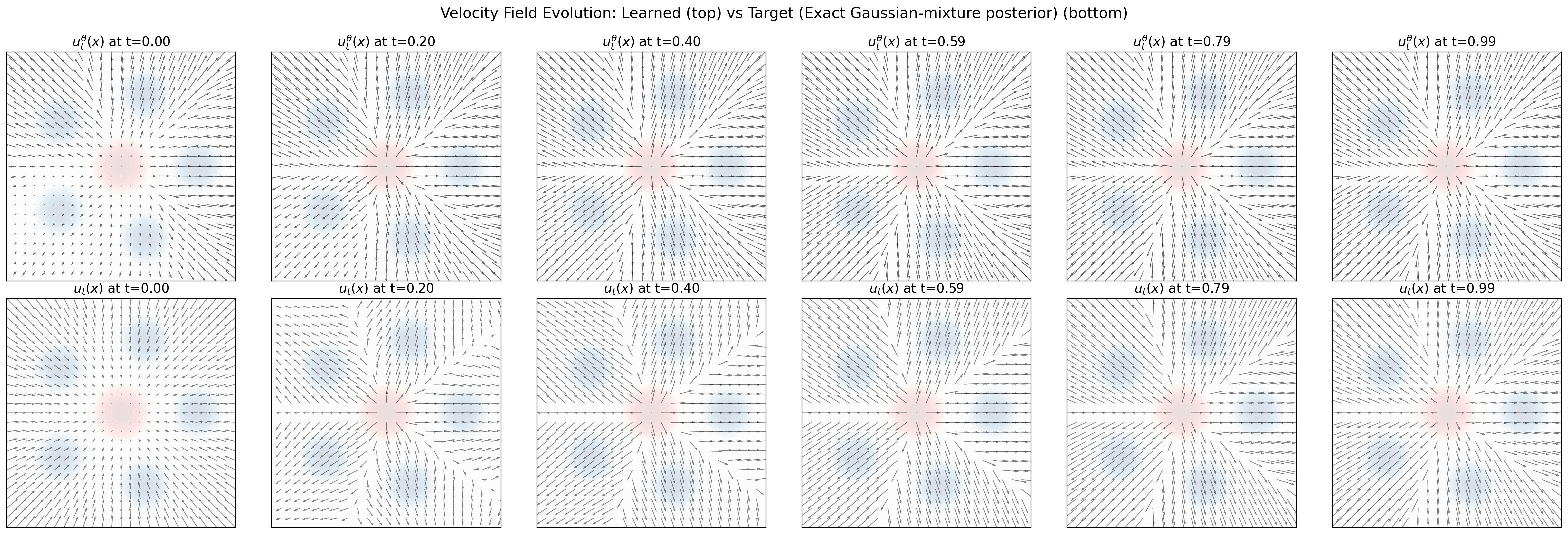
Figure 1 compares the learned vector field \(u_\theta(x,t)\) with the exact marginal field \(u_t(x)\). This is the right comparison: although the model is trained with conditional labels, the target field is the posterior-averaged marginal velocity.
At early times, the state \(X_t\) is dominated by the Gaussian reference noise. Because the data mixture is symmetric, the marginal field has a nearly radial structure. As time increases, the posterior \(p_t(z\mid x)\) becomes more informative, and different regions of the plane become associated with different mixture components. The marginal velocity then begins to split toward the five data modes.
At late times, points near a component have a posterior that is concentrated mostly on that component. The velocity field is then governed by local posterior assignment. The learned field captures this qualitative transition well: source-like behavior near \(t=0\), splitting at intermediate times, and component-wise behavior near \(t=1\).
FM/CFM loss decomposition along time
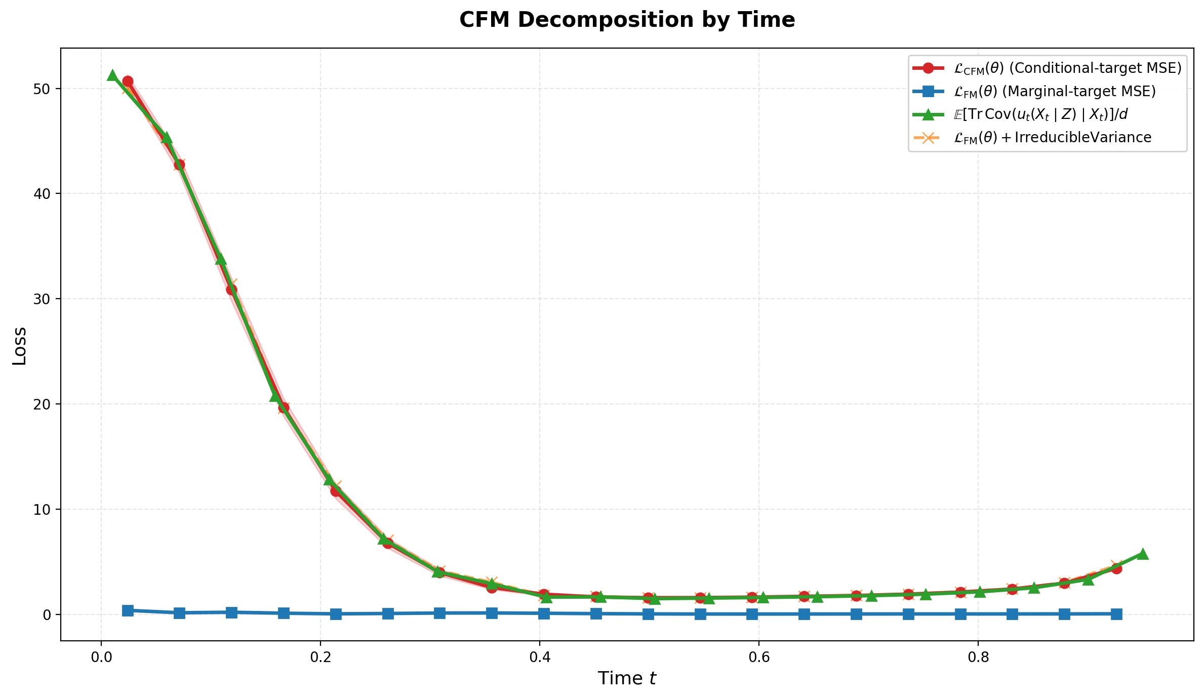
Figure 2 is the cleanest empirical confirmation of the theory. The red curve is the CFM loss, the blue curve is the FM loss against the exact marginal target, and the green curve is the irreducible variance term. The orange curve is the sum of the blue and green curves.
The key observation is that the orange curve tracks the red curve closely. This is the fixed-time decomposition in action: \[ \ell_{\mathrm{CFM}}(t;\theta) = \ell_{\mathrm{FM}}(t;\theta)+V(t). \] Moreover, the blue FM error is small for most of the time interval. Most of the CFM loss is therefore not model error; it is irreducible conditional-label variance.
The shape of the green curve has a posterior interpretation. At small times, \(X_t\) is still close to Gaussian noise and does not identify the endpoint \(Z\) well. The posterior \(p_t(z\mid X_t)\) is broad, often multimodal, and the CFM/FM gap is large. At intermediate times, \(X_t\) becomes more informative about \(Z\), so the posterior uncertainty shrinks and the gap decreases. Near the terminal time, posterior uncertainty continues to shrink, but the coefficient \(c_t^2\) grows rapidly for the schedule \(\beta_t=\sqrt{1-t}\). This terminal weighting can make the irreducible variance increase again.
Training loss
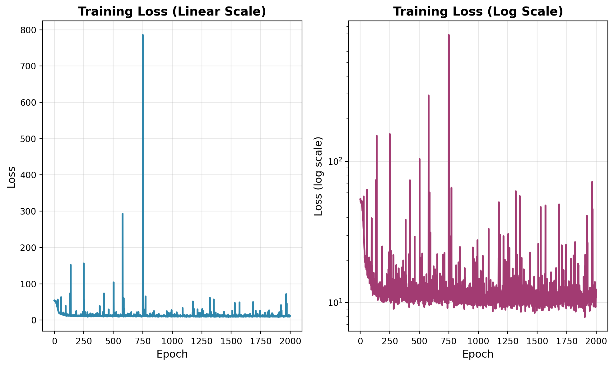
Figure 3 shows the training loss. The loss drops quickly at the beginning, indicating that the model learns the coarse transport geometry early. After that, the curve fluctuates around a lower level, with occasional large spikes.
The spikes are expected for this schedule. Since \[ u_t(X_t\mid Z) = Z-\frac{\varepsilon}{2\sqrt{1-t}}, \] minibatches containing times very close to \(1\) can produce large conditional targets and large gradients. The log-scale plot is therefore the more informative diagnostic for the late phase: it shows the overall plateau while still displaying the intermittent spikes.
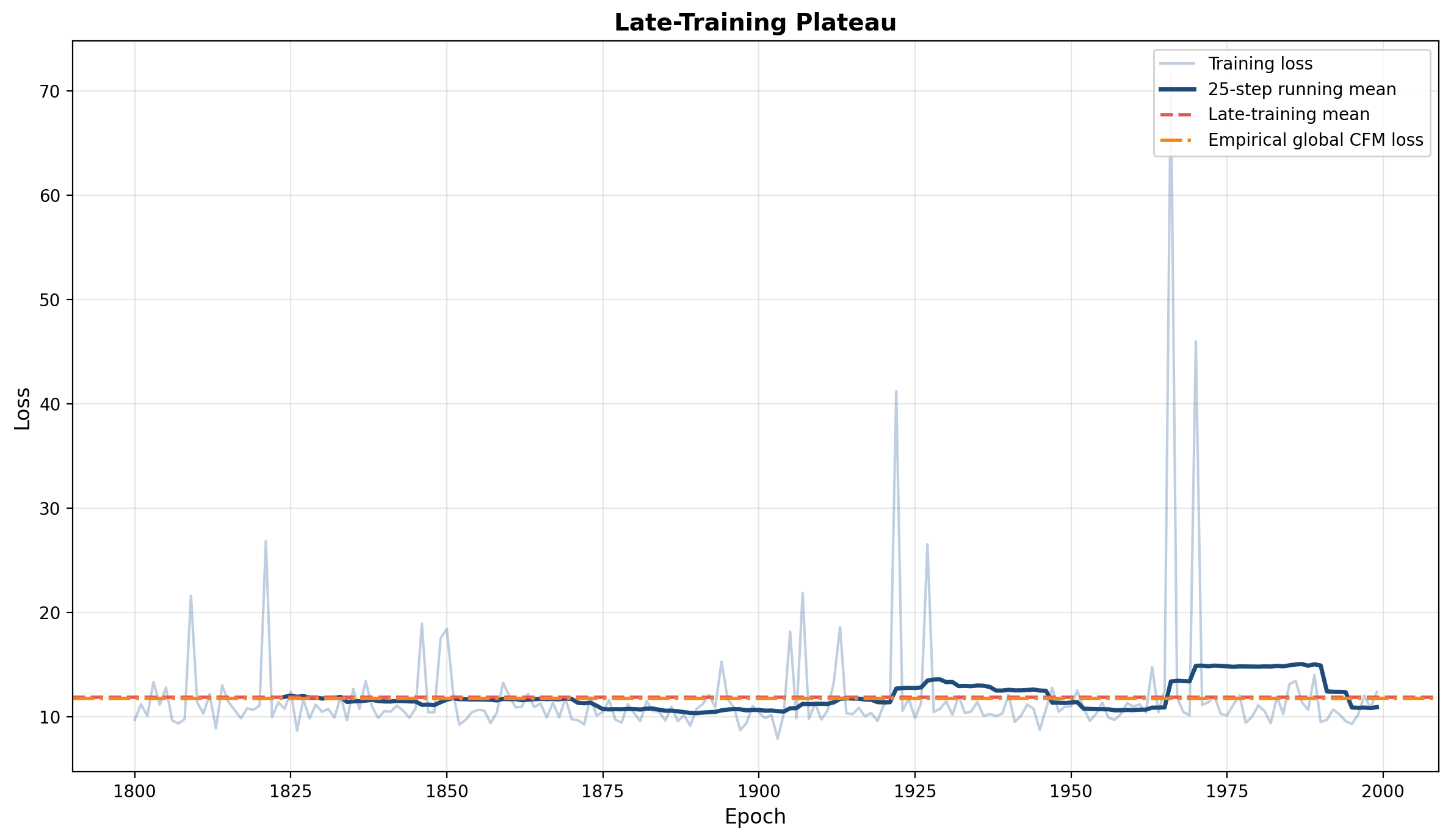
Figure 4 zooms in on the late-training regime. The smoothed training loss fluctuates around the empirical global CFM loss. This is the relevant comparison for the observed plateau, because the model is trained against conditional labels. The decomposition in Figure 2 explains why that plateau is not expected to approach the FM error alone: the CFM objective contains the irreducible variance term.
Posterior samples along random trajectories
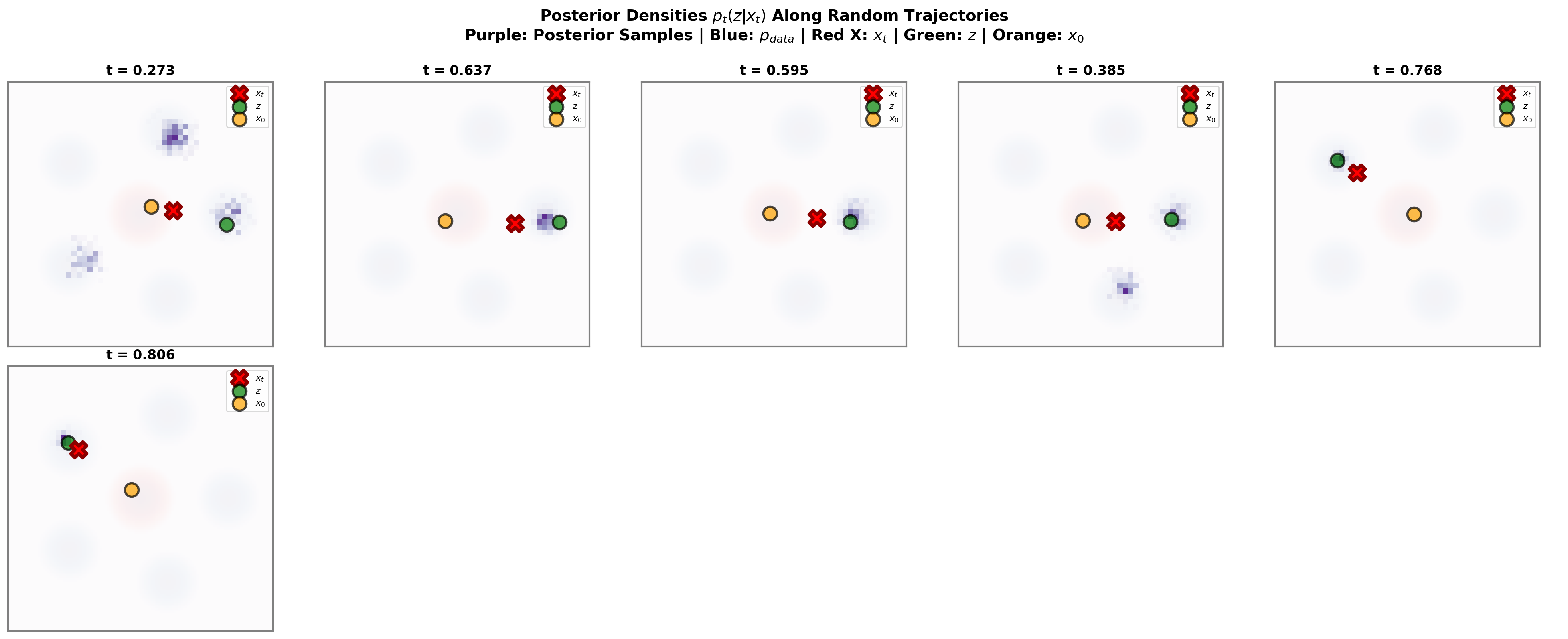
Figure 5 visualizes the posterior \(p_t(z\mid x_t)\) along randomly selected trajectories. The purple histograms show MCMC samples from the posterior, while the red cross, green marker, and orange marker show the intermediate state \(x_t\), endpoint \(z\), and source sample \(x_0\).
The main message is geometric. At moderate times, several mixture components can remain plausible endpoints for the same observed \(x_t\). In that regime, the marginal velocity is a genuine posterior average over possible endpoints, and the conditional label \(u_t(x_t\mid z)\) can be noisy relative to its conditional expectation.
At larger times, \(x_t\) usually lies closer to its endpoint, and the posterior concentrates around the correct component. The endpoint ambiguity decreases. However, the CFM/FM gap is not controlled by posterior covariance alone; it is weighted by \(c_t^2\). With the present schedule, this weighting grows near \(t=1\), which explains why terminal-time behavior remains delicate even when the posterior is concentrated.
Because the posterior is multimodal, MCMC should be read here as a visualization tool rather than as the most reliable estimator. In this Gaussian-mixture example, the exact posterior formulas above provide the benchmark. Importance sampling from \(p_{\mathrm{data}}\) is also effective because the proposal already covers all mixture components.
Appendix: posterior inference methods
The Gaussian-mixture formulas make the marginal velocity exactly computable in the running example. The methods in this appendix are nevertheless useful because they apply more broadly, when the posterior \(p_t(z\mid x)\) is not analytically tractable.
Importance sampling for posterior averages
Fix \((x,t)\) and write \[ \pi_t(z;x)=p_t(z\mid x) \propto p_t(x\mid z)p_{\mathrm{data}}(z). \] For any integrable function \(f_t(x,z)\), the posterior expectation is \[ I_t(x) = \mathbb{E}_{\pi_t(\cdot;x)}[f_t(x,Z)]. \] For the marginal velocity, \[ f_t(x,z)=u_t(x\mid z). \]
Let \(q(z)\) be a proposal density whose support contains the posterior support. Draw \[ z^{(1)},\ldots,z^{(K)}\overset{\mathrm{iid}}{\sim}q. \] The self-normalized importance weights are \[ \tilde w_k(x,t) = \frac{p_t(x\mid z^{(k)})p_{\mathrm{data}}(z^{(k)})}{q(z^{(k)})}, \qquad w_k(x,t) = \frac{\tilde w_k(x,t)}{\sum_{\ell=1}^K\tilde w_\ell(x,t)}. \] The estimator is \[ \widehat I_t(x) = \sum_{k=1}^K w_k(x,t)f_t(x,z^{(k)}). \] It is consistent as \(K\to\infty\), although it is biased at finite \(K\) because of the random normalization.
A natural proposal in this setting is \[ q(z)=p_{\mathrm{data}}(z). \] Then the prior terms cancel and \[ \tilde w_k(x,t)=p_t(x\mid z^{(k)}). \] For Gaussian paths, \[ \log \tilde w_k(x,t) = -\frac{1}{2\beta_t^2}\|x-\alpha_tz^{(k)}\|^2+C(x,t), \] where \(C(x,t)\) is independent of \(k\). The weights should be computed in log-space and normalized with a softmax for numerical stability.
A useful diagnostic is the effective sample size \[ \operatorname{ESS}(x,t) = \frac{1}{\sum_{k=1}^K w_k(x,t)^2}. \] If a few weights dominate, the estimator has high variance. In the Gaussian-mixture example, sampling from \(p_{\mathrm{data}}\) works well because the proposal already allocates mass to all relevant modes.
Markov chain Monte Carlo
Another strategy is to sample from \[ \pi_t(z;x)\propto p_t(x\mid z)p_{\mathrm{data}}(z) \] with a Markov chain. If \[ z^{(1)},\ldots,z^{(K)} \] are approximate posterior samples after burn-in, then \[ \widehat u_t^{\mathrm{MCMC}}(x) = \frac1K\sum_{k=1}^K u_t(x\mid z^{(k)}) \] approximates the marginal velocity.
The simplest option is random-walk Metropolis. Given the current state \(z\), propose \[ z'\sim\mathcal{N}(z,\sigma_{\mathrm{prop}}^2I_d) \] and accept with probability \[ \alpha(z\to z') = \min\left\{1,\frac{\pi_t(z';x)}{\pi_t(z;x)}\right\}. \] This method is easy to implement and requires no gradients, but it can mix slowly when the posterior is multimodal.
When gradients are available, MALA can be more efficient locally. The posterior score is \[ \nabla_z\log \pi_t(z;x) = \nabla_z\log p_t(x\mid z)+\nabla_z\log p_{\mathrm{data}}(z). \] For the Gaussian path, \[ \nabla_z\log p_t(x\mid z) = \frac{\alpha_t}{\beta_t^2}(x-\alpha_tz). \] MALA proposes \[ z' = z+\frac{\varepsilon}{2}\nabla_z\log \pi_t(z;x)+\sqrt{\varepsilon}\,\xi, \qquad \xi\sim\mathcal{N}(0,I_d), \] with the corresponding asymmetric Gaussian proposal corrected by a Metropolis-Hastings accept-reject step.
MCMC is flexible because it only needs the posterior density up to a normalizing constant. Its limitation is mixing. In multimodal problems, a chain may remain in one mode for a long time. Multiple chains, trace plots, and comparisons with importance sampling or exact formulas are useful diagnostics whenever they are available.
For approximately Gaussian posteriors, a rough posterior scale is \[ \sigma_{\mathrm{post}}(t) \approx \frac{1}{\sqrt{1+(\alpha_t/\beta_t)^2}}. \] This suggests initial tuning values such as \[ \text{MALA step size}\approx 0.3\,\sigma_{\mathrm{post}}(t), \qquad \text{Metropolis proposal std}\approx\frac{2.4}{\sqrt d}\,\sigma_{\mathrm{post}}(t). \] These are only starting points. The actual tuning should be checked against acceptance rates, effective sample sizes, and visual diagnostics.
References
Citation
@online{brosse2026,
  author = {Brosse, Nicolas},
  title = {Flow {Matching} as {Posterior} {Averaging}},
  date = {2026-05-12},
  url = {https://nbrosse.github.io/posts/intro-fm-diffusion/intro-fm-diffusion.html},
  langid = {en}
}